AM-ME: Analyze Quantitative Data

Development of the AM-ME was an iterative, continuous improvement process that occurred in collaboration with the research group and was informed by quantitative and qualitative analyses, content expertise, and student and staff input.  This page describes the three main types of quantitative analyses that were used to inform the development and initial validation of the AM-ME: descriptive analysis, factor analysis, and Rasch analysis.

Descriptive analyses

Simple descriptive analyses (such as means and percentages) can be a quick and easy way to help us understand how students, on average, respond to the survey items. Many surveys use mean scores (averages). However, because the AM-ME response scale is 1 = strongly disagree, 2 = disagree, 3 = agree, 4 = strongly agree, the statement that ‘students on average reported 3.06 (out of 4) in response to “I think I am good at math”’, is not easy to interpret. Rather than using the mean or average, our Research Group found it valuable to know what percentage of students agreed and strongly agreed with each of the survey items. For example, 82 percent of the students who took the AM-ME survey (strongly) agreed to “I think I am good at math”.

Key considerations for descriptive analyses

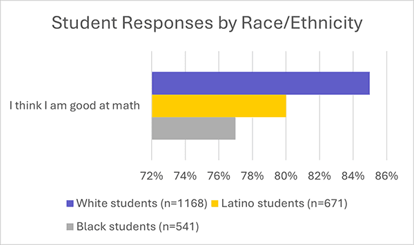
When generating descriptive statistics, an important thing to consider is how to further ease interpretation. One way to do this is to put numbers into real-world examples. If 82 percent of students think they are good at math, it might be helpful to add, “in other words, about four out of every five students who responded to our survey thought they are good at math”.  Another way to support interpretation is to provide data visualizations. We showed the percentage of students who agreed to items using bar charts (see sample below) that allowed the research group to easily see differences in how students responded to items.

Another thing to consider is whether you should disaggregate the data to examine group-level differences (e.g., rural vs. non-rural, students with or without an Individualized Education Program). A main goal of our study is to center the experiences of Black and Latino students, so we also ran descriptive analyses by race/ethnicity and tested group differences using ANOVA (with Bonferroni post hoc test to adjust for multiple comparisons). For example, we provide the following results and interpretation for the same question, “I think I am good at math”. It is important to note that it is good practice to not report disaggregated data if a group size is less than 10, since it might provide identifying information about a respondent.

Sample visualization

Factor analyses

Factor analysis is a data-reduction approach that aims to identify a set of factors (i.e., attributes or constructs) from a larger set of questions or items within a dataset. For example, in a survey on math engagement, the questions “I use math in my life” and “Math will help me in the future” might both be measures of underlying belief that math is relevant. When designing a new measure, factor analysis allows us to accomplish three main goals: 1) identify what factors exist in the data, 2) test how well the proposed factors align with responses, and 3) determine whether the proposed factors work equally well for all students. This is accomplished through exploratory factor analysis (EFA), confirmatory factor analysis (CFA), and tests of measurement invariance.

Exploratory Factor Analysis

In EFA, the goal is to identify the underlying factor structure of a set of items, as we do not yet know how many underlying factors best represent the observed patterns in the data. In EFA, we assume that each item is potentially correlated with every factor, and that the correlation between items is due to shared relationships with an underlying factor. Traditionally the number of factors is determined by examining the amount of variance each factor explains, which is measured by its eigenvalue and visualized in a scree plot. We then select the minimum number of factors needed to account for most of the variance. There are no strict rules for deciding the number of factors. Finally, when factor analysis is conducted, the output includes a list of items that support each factor, and a list of factor loadings, which show how strongly each item is related to each factor.

Confirmatory Factor Analysis

The goal of CFA is to test a pre-specified model and confirm its fit with the data, which provides evidence of both the validity and reliability of the proposed measure. Following an EFA, it tests how well the proposed factor structure represents the reality of the data. CFA imposes the model chosen by the researcher on the data and then calculates measure of “goodness of fit” that can be used to quantitatively determine if the proposed factor model accurately represents the data.  Goodness of fit measures considered in this analysis included Comparative Fit Index (CFI), Tucker-Lewis index (TLI), and root mean-squared error of approximation (RMSEA).

Measurement invariance

Another key consideration for the design of a scale is making sure that it works equally well for all students. Measurement invariance is a formal way of testing if the proposed factor structure of our data fits equally well for different groups. In the development of the AM-ME scale, we were interested in developing a culturally sustaining measure that worked equally well for students of all races. There are three levels of measurement invariance: configural, metric, and scalar. Configural invariance refers to comparisons of how well the overall fit (i.e. the proposed factors) of the model varies between groups of interest. This is accomplished by comparing the fit indices of the single group model to a model that allows all parameters (factor loadings, intercepts, etc.) to vary by group membership. Metric invariance is a stricter form of invariance which asserts that not only is the configuration of factors similar across groups, but the actual factor loadings (that is, the relationship of the individual items to each factor) are similar. Finally, scalar invariance is used to test whether the intercepts of the model are similar for each group. Note that it is often impossible to meet the strictest standards of invariance, many validated and published scales only achieve partial invariance. The goal with measurement invariance is for each level to have a similar model fit as the initial model (single group).

Key considerations for factor analysis

There are many analytic decisions that must be made in conducting a factor analysis. Some of the key decisions our team made during the analytic process for the development of the AM-ME scale were:

• Using separate samples for exploratory and confirmatory factor analysis. To improve the validity of the confirmatory factor analysis results we split the sample into two random halves, one of which was used for exploratory analysis and the other for confirmatory analysis.
• Treating Likert items as ordinal. Although some debate remains in the literature, we felt that the consensus supports treating Likert items as ordinal (rather than continuous).
• Selecting diagonally weighted least squares (WLSMV)as the estimator. Due to the decision to treat Likert items as categorical, we chose WLSMV estimator.
• Treating .35 as the threshold. Selection of the appropriate threshold to consider a variable related to a factor largely depends on convention in your field of study. For this study we decided that any item with a loading of at least .35 was related to that factor.
• Removing items that are cross loaded. Items that cross-loaded (i.e. were statistically significantly related to more than one factor) were removed.
• Not conducting missing data imputation. In our sample, almost all missing data was the result of the planned missingness design, and data imputation is not traditionally done for exploratory factor analysis, we chose not to do imputation.
• Choosing oblique rotation (specifically, geomin) for exploratory analysis, which allows the factors to be correlated with one another.

Rasch analyses

Rasch analysis is part of a family of statistical methods based on Item Response Theory (IRT) and is best understood in contrast to Classical Test Theory (CTT), which is more commonly used.

Both IRT and CRT make the following assumption:

In this equation, the observed score for person i (O_i) reflects their true score (T_i) plus error (E_i). In other words, a score on a math test may reflect my knowledge in math plus my test anxiety, which may result in an observed score lower than my true score. However, CTT assumes that error is randomly distributed across individuals and therefore sums to zero.  This leads to the assumption that the average score (Ō) is an accurate representation of the measured attribute. As such, measures of reliability and validity that align with CTT focus on measure-level (or test-level) information (e.g., Cronbach’s alpha).

IRT does not assume that error across items sums to 0. It assumes that error varies across levels of the latent trait (e.g., math ability, student engagement). This shifts our focus to item-level information because the more information we have, the less likely responses reflect measurement error. It forces us to ask questions such as:

• Do we have items (sources of information) across all levels of the latent trait?
• How well do items on the test align with students' ability?
• Are some easier or harder for students?
• Do some items work differently for certain groups of students?

Why use Rasch analysis?

Using a Rasch approach supports measurement development by helping education researchers and practitioners think critically about the relationship between person ability (or level of engagement) and item difficulty (or item endorsement). For Likert scale measures, like the AM-ME, a rating scale model can be used such that:

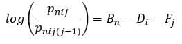
Where B_n is the location of person n on the latent construct, D_i is the average location of item i on the latent construct and F_j are thresholds for the j categories in the Likert scale. The left side of the equation is the log ratio between the probability of person n selecting category j on item over the probability of the same person selecting the next lower category on that same item. This illustrates that both person and item locations are estimated, on a similar logit metric, to allow for comparisons. In short, higher numbers represent higher locations (greater person ability, harder items) and lower numbers represent lower locations (lower person ability, easier items) on the latent construct. This information can complement reliability and validity information gleaned from measure-level analyses and inform the continuous improvement process.

Key considerations for Rasch analysis

The first consideration when conducting Rasch analyses is to determine whether model requirements of unidimensionality, local independence, and equal discrimination are met.

For the AM-ME, further considerations can be categorized into two buckets: informing the development and iterative improvement of the AM-ME, and examining the reliability and validity of the final version of the AM-ME.

Informing the Development and Iterative Improvement of the AM-ME

Two key indicators informed the development and iterative improvement of the AM-ME subscales:

• Item-Person Targeting: Refers to the alignment between item and person locations along the latent construct (math engagement subscale). The goal is to have items located in similar positions as students. In multiple iterations of the AM-ME, items targeted students at lower engagement levels. This suggested that there is greater measurement error and less precision at higher levels of engagement.
• Differential Item Functioning (DIF): Refers to items having different locations (being easier or harder to endorse) for individuals of equal ability. For example, a math question about wavelength and frequency that relies on an ocean analogy may be more difficult for groups of students that are less likely to have experienced the ocean. As a result, they may be more likely to answer incorrectly despite having an equal math ability as students who regularly experience the ocean. Assessing DIF helps ensure that the measure is fair across groups. We focused on examining DIF by race/ethnicity.

Examining the reliability and validity of the final AM-ME.

Item-person targeting and DIF were also examined to demonstrate the reliability and validity of the final AM-ME. Two additional indicators were also examined:

• Test Information Function (TIF): Refers to the extent to which a measure differentiates between individuals at different ability levels. It reflects the amount of statistical information, or precision, across the latent trait and is why it is important to have items (sources of statistical information) target individuals along the trait.
• Standard Error of Measurement (SEM): Refers to the uncertainty, or imprecision of the measure. It is inversely related to TIF.

In general, higher TIF/lower SEM suggests that the measure is reliable (the test is measuring the range of ability accurately). A broader range of TIF across ability levels suggests that scores are valid (leading to valid interpretations of scores) across the latent trait.