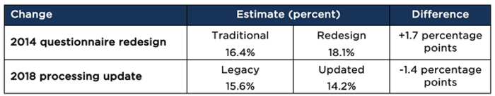
Note: These estimates are based on the assumption that the adjustment for the changes to the SPM estimates based on these two changes is equivalent with the anchored and non-anchored SPMs.

 Sources: U.S. Census Bureau, Current Population Survey, 2010 to 2022 Annual Social and Economic Supplements (CPS ASEC); and Rothbaum, J., & Edwards, A. (2019). Survey redesigns make comparisons to years before 2017 difficult. U.S. Census Bureau. 

---

Adjusted child poverty rates over time, as measured by the anchored historical SPM

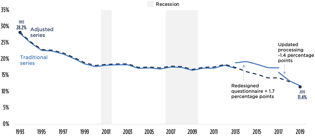
Notes: The adjusted series line (dashed dark blue) reflects adjustments for the implementation of redesigned income questions and an updated CPS-ASEC processing system. These adjustments require the assumption that the impact of the data improvements would have been identical in all years, an assumption that is less likely to be accurate in years further away from these methodology changes. These estimates are also based on the assumption that the adjustment for the changes to the SPM estimates based on these two changes is equivalent with the anchored and non-anchored SPMs.

Sources: Child Trends’ analysis of the historical Supplemental Poverty Measure data from the Columbia Center on Poverty and Social Policy. Recession data are from the National Bureau of Economic Research. Information on the adjustments come from the U.S. Census Bureau, Current Population Survey, 2010 to 2022 Annual Social and Economic Supplements (CPS ASEC); and from Rothbaum, J., & Edwards, A. (2019). Survey redesigns make comparisons to years before 2017 difficult. U.S. Census Bureau. 

---

Quantifying the role of economic factors in explaining the decline in child poverty over time using fixed effects

Our research examined the role of multiple forces—economic change, demographic change, and the growth of government assistance to low-income families—in the decline in child poverty. To assess the role of economic and demographic changes, we used two-way fixed effects regressions. Fixed effects is a widely accepted statistical methodology and, in applying it here, we are adapting methods used by Hilary Hoynes, Marianne Page, and Ann Huff Stevens in the 2006 article Poverty in America: Trends and Explanations. This method allows us to explore the year-to-year variation among states in economic indicators such as states’ economic growth in GDP, states’ minimum and median wages, and single mothers’ labor force participation rates; and in demographic indicators such as the share of children in two-parent families, the share of adults with a high school degree or higher, the racial and ethnic composition of the child population, the share of children living in immigrant families, and teen birth rates. We capitalize on variation in the timing and extent of these state-level changes in economic and demographic factors in order to estimate the extent to which changes in these indicators are associated with changes in child poverty rates. Looking at state-level changes allows us to more rigorously examine the role of economic and demographic factors because differences between states can operate like a comparison group: If one factor changes in one state but not in another (or to a different degree in another), then we can estimate the impact of that change in one state, compared to its impact in the other.

Our models include both state and year fixed effects. The strength of this methodology is its ability to first eliminate the impact of unobserved variables that are common to all states (omitted variable bias). Take the example of states experiencing technological advances in high-speed internet: These states may see both increases in GDP (via a common improvement in productivity) and decreases in child poverty (via increased access to information about safety net programs via the high-speed internet connections). A model without year fixed effects might overestimate the role of GDP because it also captured the omitted variable (technological advances in high-speed internet). Second, the state-level fixed effect effectively removes any problematic unobserved heterogeneity that is time-invariant within a state (meaning, it controls for any fixed factors explaining differences in child poverty rates across states). Failing to control for unobserved variables risks skewing the analysis.

But there are trade-offs to using fixed effects models. One drawback is that we remove the influence of changes that occur at precisely the same time and degree in every state. However, while a fixed effects model would not capture the influence of changes that occurred everywhere at the same rate, even large national trends like economic growth generally happen at different degrees, in different places, and with different timings. It is that variation on which we capitalize.

Because this methodology does not capture changes that occur simultaneously across states, it may underestimate some of the economic changes propelling the decline in child poverty, such as wage growth or increased work effort among single mothers. But other elements of our design lean in the opposite direction, potentially overstating the role of such factors. Across our study, we examined changes in child poverty from a time of economic weakness (1993) to one of economic strength (2019). These beginning and end points (chosen for other reasons, which we explain in our report) may put additional emphasis on economic growth and understate the role of the social safety net in the decline in child poverty.

Taking a step back from the analysis in our report, we can compare declines in pre-tax-and-transfer (PTT) child poverty to SPM child poverty to get a general sense of how earned income—which may increase with a healthy economy—declined over time compared to SPM poverty. Using the anchored historical SPM data, and looking at the decline in child poverty from 1993 to 2019 (again, from a time of economic weakness to economic strength), we saw a decline in PTT poverty of 34 percent and a decline in SPM poverty of 59 percent. If, instead, we were to look at the decline between two periods of economic strength (e.g., from 1989 to 2019), PTT poverty would have declined by a smaller 24 percent and SPM poverty by 54 percent. Taking this approach (which some have argued is more fair) indicates additional growth in the role of the social safety net.

We should also note that our study was not designed to measure behavioral interactions between the social safety net and demographic or economic factors (e.g., whether individual programs pushed people into work and increased their incomes via this push). Other researchers have done great work on this question. See, for example:

• Gibson et al., 2017: https://www.cochranelibrary.com/cdsr/doi/10.1002/
  14651858.CD009820.pub2/full
• Gray et al., 2021: https://www.nber.org/system/files/working_papers/
  w28877/w28877.pdf
• Grogger, 2001: https://www.nber.org/system/files/working_papers/
  w8153/w8153.pdf
• Wu et al., 2008: https://academic.oup.com/swr/article-abstract/32/2/89/1620774

---

Quantifying the role of the social safety net in reducing child poverty using the CPS-ASEC

We took a different approach to quantifying the role of the social safety net in reducing child poverty—one that is not comparable to the fixed effects method described above. The state-level fixed effects methodology is not suitable for analyzing the impact of changes in the federal social safety net, such as the growth of the Supplemental Nutrition Assistance Program (SNAP) or tax credits, since those changes largely occur at the same time across the country. Instead, we followed established precedents—namely, the methods that the Census Bureau uses in its annual SPM reports: We calculated SPM child poverty rates with and without the social safety net by subtracting out the cash value of government benefits from the resources available to a family. Again, because we used different methodologies in assessing the safety net, we cannot directly compare the share of poverty reduction that came from government aid versus the share influenced by other forces. We conclude only that the safety net played an essential role.

As we thoroughly document and note in our study, the CPS-ASEC data underestimate some safety net benefits due to underreporting of benefits in surveys and overestimate the role of the Earned Income Tax Credit (EITC). The EITC values are simulated, and they are not perfect. The simulation is based on family income, family structure, and family composition, and does not account for the approximately 20 percent of tax filers who are eligible for, but do not claim, the EITC. Nor does the simulation account for workers who do not routinely file taxes because they have no tax liability, but who are nonetheless eligible for—and would otherwise receive—the EITC if they were to file taxes. The simulation also does not account for any fees that paid tax preparers may charge.

But while Census methods overstate the support that families receive from the EITC, they understate the resources families received from SNAP and TANF (Temporary Assistance to Needy Families). To a substantial degree, these methodological weaknesses counteract each other, although the net effect to overstate or understate poverty rates is not clear.

Some researchers try to correct these known inaccuracies by correcting the data, particularly for underreporting (with more simulations, which require yet more assumptions). However, the current most frequently used microsimulation, TRIM3, does not cover the full range of years included in this report (L. Wheaton, personal communication, April 19, 2022). For now, we have used the best data available, while noting the limitations.

---

The big picture

Methodological choices are critical to the quality of any research, and debates about those choices are fundamental to the research process. We are transparent about our approach and aim to be as rigorous as possible. Intellectual debate is important when it moves the field forward—and we’re all in this field to help children.

As a country, we have imperfect ways of measuring poverty and assessing the reasons behind its decline. But those imperfections do not change the conclusions we reached in our study. The United States has seen an astounding drop in child poverty over the last 25 years, and the safety net and a healthy economy worked together to contribute to this decline.

---

Footnote

[1] There are, of course, additional ways to measure poverty and economic hardship and all of its various harms. It’s always good to look across these measures for a comprehensive picture, with the recognition that each measure reflects a different dimension of the experience of hardship and that they may not always move in tandem with the others.